Wind Turbine Controllers / Fast and Simulink
A tutorial on how to simulate Wind Turbine controllers using NREL's Fast and Matlab/Simulink
Project maintained by borgestassio Hosted on GitHub Pages — Theme by mattgraham
Linearization
In this section we cover the Linearization using Fast V7 (Files and short guide available here: https://github.com/borgestassio/FASTv7). I used V7 simply because it’s easier to perform the linearization and I followed the instructions on FAST User’s Guide, where it explains how to achieve the linearization using the numerical pertubation method. If you want to learn more about the symbolic method, I suggest you read the Modern Control Design for Flexible Wind Turbines technical report by Alan Wright.
According to Wright:
In the numerical method, values for the mass, damping and stiffness matrices are calculated directly in FAST, during runtime. The code is first run for steady winds, i.e., no turbulence. Once a steady-state solution has been reached, the equations of motion are numerically perturbed with respect to each DOF (Degree of Freedom) and its derivative.
And quoting the FAST User’s Guide, this is what the linearization method does:
Once a periodic steady state solution has been found, FAST numerically linearizes the complete nonlinear aeroelastic model about the operating point.
I strongly suggest you to read both documents to have a better understanding of the linearization procedure.
We proceed with a simple explanation of it does before we move to how to do it.
In order to extract the state matrices, FAST reaches a stead-state solution and then adds smalls perturbations until a linear response is obtained from these perturbations. It’s important to note that the system is linearized about the Operating Point (OP) and the matrices depend on the rotor azimuth position. Therefore the matrices are periodic. The User’s guide also states:
It is important to determine an accurate operating point because the linearized model is only accurate for values of the DOFs and inputs that are close to the operating point values.
The objective of the linearization is to extract the state matrices and have the state-space representation of the Wind Turbine model:

Where:
- Δx is the state vector;
- Δu is the control input vector;
- Δu_d is the disturbance input vector;
- Δy is the control (or measured) output;
- A represents the state matrix;
- B the control input gain matrix;
- B_d is the disturbance input gain matrix;
- C relates the measured output Δy to the turbine states;
- D relates the control input to the output;
- D_d relates the measured output to the disturbance states.
That being said, we focus on how to acquire these matrices.
CONFIGURATION FILES AND PARAMETERS
For the linearization, the process will follow the instructions presented in Advanced Control Design for Wind Turbines, despite its use of a 2 bladed turbine, the process is almost the same, and for the parameters regarding the 5 MW Wind Turbine, we’ll follow Definition of a 5-MW Reference Wind Turbine, which contains all definitions and configurations of the turbine. Inside your .fst file, in this case, “NRELOffshrBsline5MW_Onshore.fst”, go to the FEATURE FLAGS (LINE 54). Now we begin to modify the configuration file to obtain the results needed, the appropriate Degrees of Freedom (DOF) will be used for the linearization:
- FlapDOF1;
- DrTrDOF;
- GenDOF;
- CompAero. The others DOFs must be set to False, so your file will look like this:

To perform the simulation, we will need to change some lines in the SIMULATION CONTROL part:
- ADAMSPREP should be set to 1 (Run FAST);
- AnalMode should be 2 (which is to create a periodic linearized model);
- NumBl remains the same, as we’re working with 3 blades;
- TMax is advised to be 1200, although the linearization will be achieved before that;
- DT is set to 0.006 for no particular reason described in any document.
The SIMULATION CONTROL portion of your file should be similar to this:

The linearization process utilizes the turbine parameters to perform the calculations, therefore, in order to successful linearize the model, we must pass to FAST the correct parameters to the turbine control, which is done in the TURBINE CONTROL portion:
- YCMode must be 0;
- PCMode is set to 0;
- VSContrl is activated, set to 1;
- VS_RtGnSp must be 121.6805;
- VS_RtTq is 43093.55;
- VS_Rgn2K is set to 2.332287;
- VS_SlPc is equal to 10.0;
- GenModel is 3;
The others parameters remain the same, so your file should be similar to this:

I might be mistaken, but I believe all other parameters are already set correctly, so it is time to move to other file, at this point, specifically to the NRELOffshrBsline5MW_Linear.dat file, where the linearization properties are.
Here, the changes are:
- VelTol to 0.00001;
- NAzimStep to 24;
- NInputs to 1;
- CntrlInpt to 4;
- NDisturbs to 1;
- Disturbnc to 1;

With these changes, the parameters are all set, however, one more thing is necessary, the wind profile. To make things easier, we will use the simplest wind profile file, a Hub-Height file, this file implements a 12 m/s wind profile, suitable for model linearization in FAST v7, Jason Jonkman made this file available in the NREL Forum in a topic about the 5 MW Wind Turbine (https://wind.nrel.gov/forum/wind/viewtopic.php?f=4&t=621). Although the file extension attached in the topic is .txt, the usual extension is .wnd. The file format is quite simple, in the file one can see that the data is divided into columns, and in this case, all we need is the time and wind speed, so the file looks exactly like this:

Along with the wind profile, we have to tell FAST which file it will use for the wind, we do this by changing the AeroDyn file (NRELOffshrBsline5MW_AeroDyn.ipt), as shown in the Figure below.

These files are in the folder Files here, so if do not want to change every file, and have trust in me, you can use the files provided here or here.
LINEARIZATION
The configuration files and wind profile must be in the same folder as the FAST executable in order to execute the simulation and find the linear model.
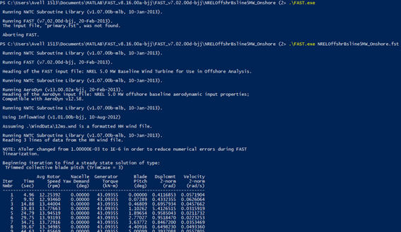
Once you have all files and the executable in the same folder, open the command prompt (Here, I assume you are using windows to makes things easier for me), or the new Windows PowerShell, directly in the folder you are currently working by holding shift and right-click, select “Open Command Window here”.
Type FAST.EXE (or .\FAST.exe ) followed by the input file, in this case:
.\FAST.exe NRELOffshrBsline5MW_Onshore.fst

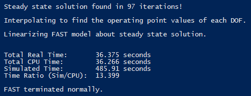
The final output should be similar to this:

POST-PROCESSING WITH MBC3
The FAST outputs the .lin file with the linearization results, to easily extract them we can use a post-processing tool, espeficially the MBC3, also developed by NREL (https://nwtc.nrel.gov/MBC and on GitHub https://github.com/NWTC/MBC).
To obtain the desired matrices we must use one function from the MBC3, I leave you to choose where to extract the files from MBC3, but make sure you execute the function in the same folder where your .lin file is located. The instructions to extract the matrices from the .lin file follows:
- Download MBC3 and extract it on your Matlab folder;
- Go to the folder where your .lin file is located;
- Execute the following command:
GetMats;
The command window on Matlab will as for the .lin file

-
Enter the name of the file without the .lin extension, in my case it is: NRELOffshrBsline5MW_Onshore
-
If everything went fine, you will see the message:

- Your matrices are now available, as described in User’s Guide to MBC3, as the azimuth-averaged state matrices:
- AvgAMat = A
- AvgBMat = B
- AvgBdMat = Bd
- AvgCMat = C
- AvgDMat = D
- AvgDdMat = Dd
Given that the linearized model is calculated only around the OP, the results for the linearized model will include not only the matrices but the OP as well. This is very important because the linear model will only represent the system around the OP, therefore the plant to be controlled is the WT working on the OP. The OP includes Rotor Speed, Pitch Angle and Wind Speed.
This means that a simple feedback controller will work best if the WT is operating close to the OP. We’ll increase the complexity of the model and its controller until we can cover all Operating region of the WT.
In possession of these matrices, you now have a linearized model that can be used to design the controllers described in Advanced Control Design for Wind Turbines. Refer to the other folders to find the guide for each type of controller.