Wind Turbine Controllers / Fast and Simulink

A tutorial on how to simulate Wind Turbine controllers using NREL's Fast and Matlab/Simulink

---

Project maintained by borgestassio Hosted on GitHub Pages — Theme by mattgraham

State Space Controllers

In here we focus solely on building the simple state space feedback controllers, this means that EVERY state is available through a sensor, which is clearly not the case for a real-world application. The goal is to start with something simple and then we move to more complex techniques.

The state space equation for a linear system has the form:

We saw how to obtain the A,B,C and D matrices from the linearization.

Now, we extract that information to create our own model and design the feedback controller.

1 State Model

Using the Lineazation guide, we get the 1 state model (single DOF - Rotor - GenDOF), we can see that the system was linearized with the following parameters for the OP:

The matricies extracted from the linearization are:

• A = -0.37035;
• B = -0.39467;
• C = 1;
• D = 0;

Note: the xop variable from the linearization includes the blade pitch on the first line and the rot speed (rad/s) in the second line, therefore only the 4th element from the AvgAMat is used here, because it’s the only element that has a direct relationship with the rotor speed The same approach will be used from now on, we’ll only use the elements from the AvgAMat that relates to the states of the model. On the .m files we’ll index them accordingly.

This is the AvgAMat:

This is the x:

I hope you can see the reason why only the element A22 on this 1-State model.

Simulation

Now we work our way to Simulink, but before we do, let’s learn a little bit more about interfacing Fast and Simulink.

* Indexing

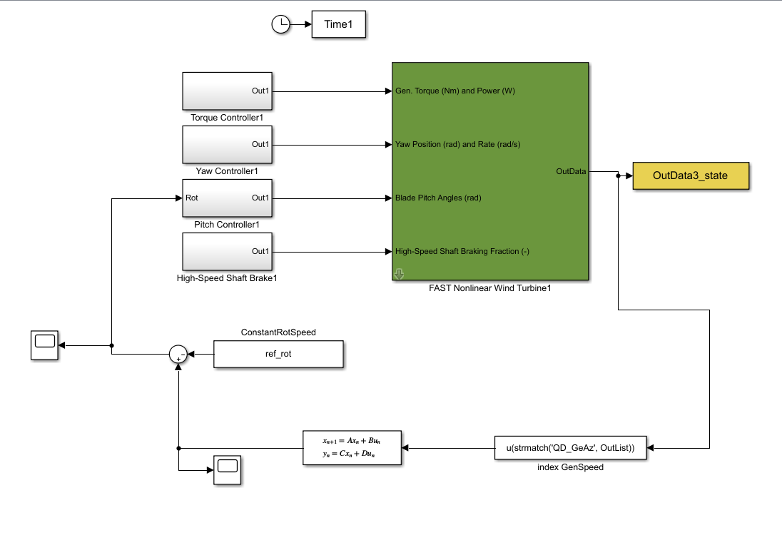
This is Simulink model (available on the files folder):

In order to index the rotor speed, a expression block is needed. Inside the block, this is the expression you should enter to get the rotor speed: u(strmatch('QD_GeAz', OutList))

The output QD_GeAz is the rotor speed in rad/s.

* Filtering

The next block is a Discrete State-Space block, where a filter is implemented. The corner frequency, defined in the Definition of a 5-MW Reference Wind Turbine for Offshore System Development, is set at 0.25Hz. On this block we implement the low-pass filter as described on the section 7.1 of the technical report.

* Implementing the controller

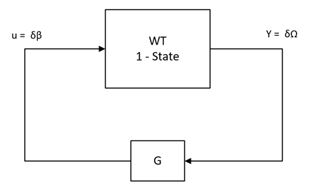
You’re well aware that the linearized system represents the WT around that specific OP, but what does it mean from the control point-of-view? It means that the system aims to keep the ‘variation’ of its states as ‘0’, therefore the input and output of this type of system is the variation from the OP. When representing on Block Diagram, the feedback controller for the 1-state system looks like this:

Here we can see that we need to pass the rotor speed variation to the controller and it’ll output the pitch variation.

On the simulink model we achieve that by subtracting the measured rotor speed from the OP rotor speed. As for the pitch, we sum the OP pitch to the controller output:

Please note the pitch is in radians, as it’s the input unit used by FAST. We have a saturation and a rate limiter block copied from the PID baseline to keep it within operation limits.

* Pole Placement

In here we implement a Full State Feedback controller. We can easily see that the pole for this system is -0.37035. You can see that using the pzmap(sys1) command after running the test_1_state.m file available here.

We’ll place the pole at -1 using the following function: pole = -1;

G = -place(A,B,pole);

It returns as G = 1.5954

You can try yourself and place the root at another location to see what it does to the response, it’s a good exercise.

* Running the simulation

The simulation is ran with the same DOFs as the linearization, in this case it’s only the rotor DOF.

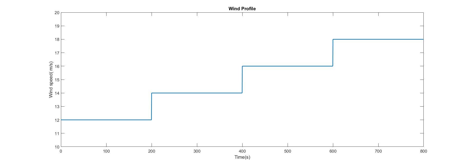
The wind profile used for all the simulations here is a 2 m/s step from 12m/s to 18m/s:

You just need to press play and wait for the simulation to finish. On the 1_state.m file you’ll find some commands to print the results:

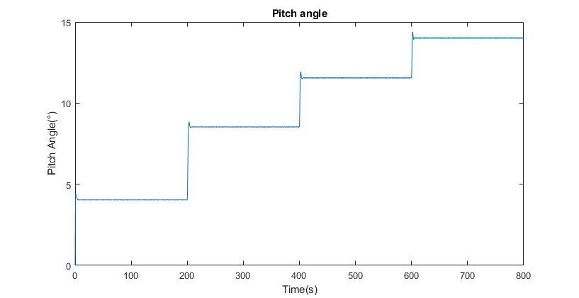
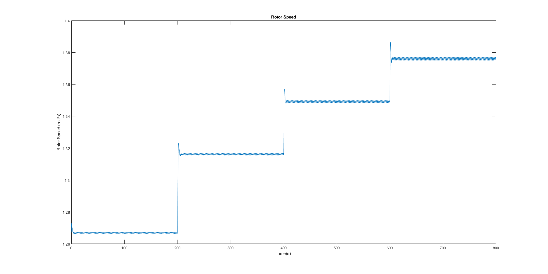
We can see that while the wind speed is 12 m/s, i.e. OP, the rotor speed is also kept around the OP (1.26 rad/s).

You can find all the data on the variable named Outdata and the list of ouputs on OutList.

3 States Model

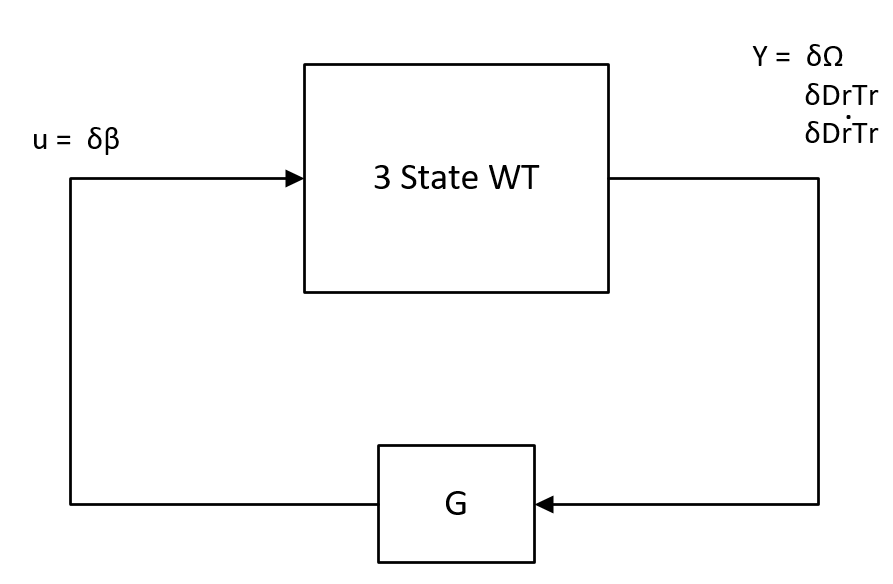
In this model, we enable the torsional flexibility of the drivetrain (DrTr DOF). We use the DrTr and its derivative to create the 3 State Model:

This is the state space representation:

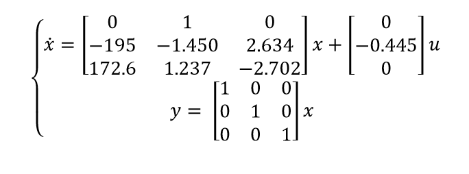
In the control_3_states.m file, we have the code to index the matrices, and we also have some commands to run the LQR and find the poles that way.

I decided, arbitrarily, to place the roots at -1, -6+13.816i and -6-13.816i Once again, you can play with those or try the LQR technique to change the gains and behaviour of the system.

Note that we’re dealing with a full state feedback, therefore we have to provide all the states to the controller.

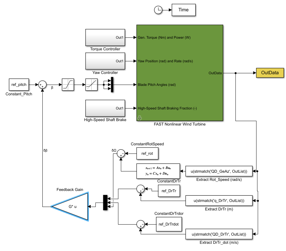
The simulink diagram should look like this:

Where you can see that we extract all 3 states and pass them to the feedback controller.

You can run the simulation using different pole placement values and even the LQR technique to see how the system responds.

5 States Model

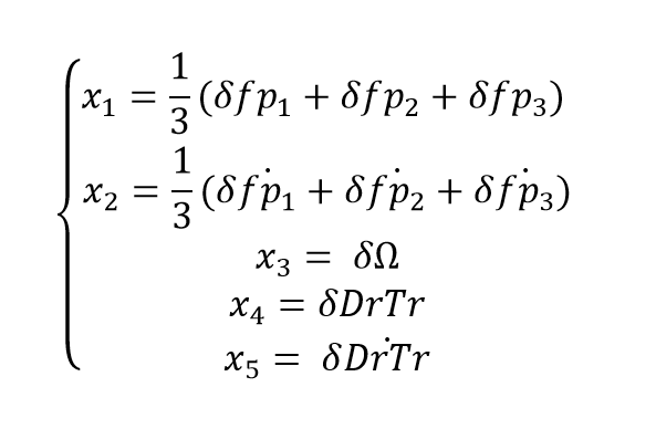
For this model, we add the flapwise DOF, which in turn adds 2 states for each blade: 1st flapwise bending deflecion mode and 1st flapwise bending velocity. Therefore, a total of 6 states are added to the model. This results in a non-controllable and non-observable system. The solution, proposed by Wang et al (2016), is to explore the symmetrical and asymmetrical effects of the blades on the rotor. This allows the states to be transformed in the symmetrical and asymmetrical rotor flap bending. Please note that on the Collective Pitch Control (CPC), the asymmetrical mode is not used, given that the system will only controlable when using the Individual Pitch Control (IPC) method, we’ll get to that later. The manipulation of the states follows:

Using these states and the CPC method, the system is observable and controlable.

As usual, you can find the .lin, the .m and the Simulink Model on the files folder In the .m file you’ll find the implementation of this manipulation after indexing the states from the linearized system.

I used the LQR to find the feedback gain, but you can change that and use pole placement. Please note that on the same file there are some parts commented that achieve other objectives that we’ll see later.

Alright, it’s time to move to state observers now because we’ll keep adding states that are unable to being measured. See the next section to continue this tutorial.